3.2 Inelastic excitations: coupled channels method

We consider the scattering of a projectile a by a target A. We denote this partition by the index $\alpha$, i.e., $\alpha=a+A$. The Hamiltonian of the system is expressed as:

$$H=H_{\alpha}+K_{\alpha}+V_{\alpha}\,\,,$$ (9)

where $K_{\alpha}$ is the total kinetic energy, $V_{\alpha}$ is the projectile-target interaction and $H_{\alpha}$ is the sum of the internal Hamiltonians, i.e., $H_{\alpha}=H_{a}+H_{A}$.

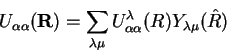
We assume for simplicity that only one of the nucleus (let's say, a) is excited during the collision and that this nucleus has only one excited state. The model wavefunction will have both elastic and inelastic components. It can be expressed as [3]:

$$\Psi=\phi_{\alpha}(\mathbf{r})\chi_{\alpha}(\mathbf{R})+\phi_{\alpha'}(\mathbf{r})\chi_{\alpha'}(\mathbf{R}),$$ (10)

where $\phi_{\alpha}(\mathbf{r})$ and $\phi_{\alpha'}(\mathbf{r})$ are ground state and excited state wave functions of the nucleus a and, hence, are solutions of the Schrodinger equation with the Hamiltonian H_a:

$$H_{\alpha}\phi_{\alpha}(\mathbf{r}) \epsilon_{\alpha}\phi_{\alpha}(\mathbf{r})$$ =

$$H_{\alpha}\phi_{\alpha'}(\mathbf{r}) \epsilon_{\alpha'}\phi_{\alpha'}(\mathbf{r}).$$ = (11)

The functions $\chi_{\alpha}(\mathbf{R})$ and $\chi_{\alpha'}(\mathbf{R})$ describe the relative motion between the projectile and target in the different internal states. The total wavefunction $\Psi$ verifies the Schroedinger equation: $(E-H)\Psi=0$. By projecting this equation onto the different internal states a set of two equations is obtained:

$$(E-\epsilon_{\alpha}-K_{\alpha}-U_{\alpha\alpha})\chi_{\alpha}(\mathbf{R}) U_{\alpha\alpha'}\chi_{\alpha'}(\mathbf{R})$$ =

$$(E-\epsilon_{\alpha'}-K_{\alpha'}-U_{\alpha'\alpha'})\chi_{\alpha'}(\mathbf{R}) U_{\alpha'\alpha}\chi_{\alpha}(\mathbf{R})\,,$$ = (12)

where $U_{\alpha\alpha}$ and $U_{\alpha\alpha'}$ are the so called coupling potentials. Thus, for example, $U_{\alpha\alpha'}$ is the potential responsible for the excitation from the initial $\alpha$ state to the final state $\alpha'$. These potentials are constructed within a certain model, as we will see later. In the coupled channel (CC) approach, the coupled equations (12) are solved exactly, to give the functions $\chi_{\alpha}(\mathbf{R})$ and $\chi_{\alpha'}(\mathbf{R})$.

If the number of states is large, the solution of the coupled equations can be a time consuming task. In many situations, however, some of the excited states are very weakly coupled to the ground state. For example, referring again to the two channels case, this suggests that the inelastic component of the total wavefunction (10) is going to be a small fraction of the elastic one. This allows to get an approximated solution of the coupled equations by setting to zero the inelastic component in the first equation:

$$(E-\epsilon_{\alpha}-K_{\alpha}-U_{\alpha\alpha})\chi_{\alpha}(\mathbf{R}) \approx$$ 0

$$(E-\epsilon_{\alpha'}-K_{\alpha'}-U_{\alpha'\alpha'})\chi_{\alpha'}(\mathbf{R}) U_{\alpha'\alpha}\chi_{\alpha}(\mathbf{R})\,.$$ = (13)

Thus, the first equation can readily solved. The resulting function $\chi_{\alpha}(\mathbf{R}$ ) is then inserted into the second equation, allowing the calculation of $\chi_{\alpha'}$. This is called 1-step distorted wave distorted wave Born approximation (DWBA). An iterative procedure can be then applied by inserting the calculated $\chi_{\alpha'}$ into the first equation in (12) to get an improved function $\chi_{\alpha}$. Continuing this procedure, we can get 2-step, 3-step, etc DWBA. When the couplings between channels are weak, the DWBA should approach to the full CC solution. However, when couplings are strong convergence problems can be presented.

As in the pure OM calculation, a separation between the angular and radial parts is made in the set of coupled equations (12). This requires the expansion of the potentials $U_{\alpha\alpha}(\mathbf{R})$ and $U_{\alpha\alpha'}(\mathbf{R})$ in multipoles. For example:

$$U_{\alpha\alpha}(\mathbf{R})=\sum_{\lambda\mu}U_{\alpha\alpha}^{\lambda}(R)Y_{\lambda\mu}(\hat{R})$$ (14)

where $\lambda$ is called multipolarity. In principle the expansion above runs from $\lambda=0$ to $\lambda=\infty$. However, in practice, only the first few multipoles play a significant role in the scattering process. With the variable IP1 (in the namelist &couplings/) we set the maximum value of $\lambda$. The specific form of the coupling potentials depend on the adopted model.

The resolution of the coupled equations (12) is significantly simplified if the distorted wavefunctions are separated into their radial ($f_{\alpha}(R)$) and angular parts. Thus, inserting the multipole expansion (14) into the coupled set of equations one gets:

$$\left[E_{\alpha}-T_{\alpha L}(R)-U_{\alpha}(R)\right]f_{\alpha}(R) \sum_{\lambda}U_{\alpha\alpha'}^{\lambda}(R)f_{\alpha'}(R)$$ =

$$\left[E_{\alpha'}-T_{\alpha'L}(R)-U_{\alpha'}(R)\right]f_{\alpha}(R) \sum_{\lambda}U_{\alpha'\alpha}^{\lambda}(R)f_{\alpha}(R)\,\,,$$ = (15)

with

$$T_{\alpha L}(R)=-\frac{\hbar^{2}}{2\mu}\left(\frac{d^{2}}{dR^{2}}-\frac{L(L+1)}{R^{2}}\right).$$